
How do professional investors decide how much to diversify? And how can you tell if your portfolio is diversified enough?
The current standard theoretical framework for diversification in investing is Modern Portfolio Theory (MPT). MPT is a way to think about the benefits of diversification, and specifically about the idea that when you mix different investments together in a portfolio, you keep the average return characteristics of all the individual assets, but you lose some of the average volatility of the same assets. So, in most cases, when you mix assets together in a portfolio, you wind up with a total investment that has more “bang for your buck” than the individual securities by themselves.
History of modern portfolio theory
Modern portfolio theory was developed by economist Harry Markowitz in the 1950s. I’ll skip the math, but if you’re interested, the linked Wikipedia pages have excellent descriptions of the theory and its derivation. But, the key concept behind MPT is very important to all investors, including you!
Why is diversification good?
All investments should be considered on a risk-reward basis. Investors don’t like taking risks, so any investment should be seen as offering some kind of trade-off between higher risk, higher return investments and lower risk, lower return investments. Markowitz recognized that investors don’t have to choose just one investment. Investors have the flexibility to combine assets into portfolios that can offer similar return characteristics to a given asset, but with reduced risk.
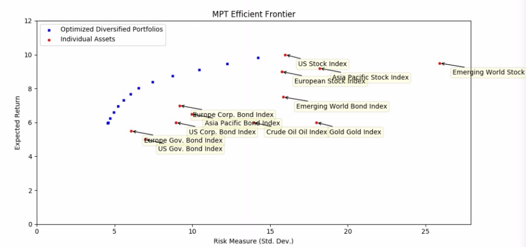
For example, in the chart below, I have used a simple portfolio optimizer developed in-house at Luther Wealth to find several diversified portfolios (blue dots) that have higher expected annual returns and lower expected volatility than any of the individual investments (red dots). In other words, assets that are located at the top left of the chart have better risk-reward characteristics.
OK, so how does diversification actually improve my risk profile?
Diversification is good, because of the different ways that individual assets contribute to a portfolio’s expected return and risk characteristics. The key insight is based on two math facts about portfolios made up of two individual assets:
- The expected return of the portfolio is the simple average of the expected returns of the two assets.
- The expected volatility (riskiness) of the portfolio is a little bit less than the simple average of the volatilities of the two individual assets. The magnitude of this “little bit” is inversely related to how closely the two assets tend to move with each other (correlation).
So, when you mix up assets into a portfolio, you “keep” the return of the assets, but you “lose” a little volatility (risk), which is good! And the less correlated the assets, the more risk falls out of the portfolio. This is the essence of diversification, and it’s the essence of modern portfolio theory.
Well known drawbacks of traditional portfolio optimizers
Sounds great, right? Well, modern portfolio theory, in practice, has several well-known drawbacks that sharply limit its application in real world investing.
MPT assumes all assets returns are normally distributed
First, in most current implementations, the optimization software forces an assumption that all assets have expected return distributions that follow a normal, or “bell” curve. This means that the software assumes any given asset has an average expected return, with variations explained and predicted by that asset’s variance, or standard deviation.
This framework means that the optimizer is forced to assume that really big gains and really big losses almost never happen. It also forces the optimizer to assume that a big gain and a big loss are equally probable on a given day. Most experienced stock market investors can tell you that this is not the case!
This drawback is not a knock on Markowitz. In fact, the general theoretical framework he developed allows all kinds of distributions to be used. However, when MPT was fleshed out from the 1950’s to the 1990’s, the available computing hardware became a limiting factor. This is because calculating portfolio standard deviations for normally distributed data is computationally simple, while calculating the same measures for non-normal distributions would have required a massive amount of computing power in the past. So in the past, the only practical option was to assume everything follows a normal distribution.
MPT assumes correlations between all assets are stable
The benefit of diversification is inversely related to the degree of correlation between each of the portfolio assets. The less correlated the constituents, the more “juice” you get out of diversifying. This makes intuitive sense. For example, consider two stocks in completely unrelated sectors. Maybe one company does better in recessions, and the other company does better in booming economies. If you hold a diversified portfolio of both stocks, big losses in one stock will tend to be smoothed out by gains in the other, reducing the volatility of your portfolio.
Here again, traditional optimizers run into a problem. Most existing financial software is limited by the fact that the software can only accept a single value for the correlation between any two assets. In other words, stock ABC and stock XYZ exhibit the same correlation in normal times, in stock market crashes, and in stock market bubbles.
Stock traders can tell you that this is a faulty assumption. Particularly during stock market crashes, all assets– stocks, bonds, commodities, etc. — tend to go all go down in a synchronized manner. In other words, during a crash, all correlations go to 100%. So traditional portfolio optimizers tend to overestimate the benefits of diversification, because when you need diversification the most (i.e. during a crash), the benefit tends to evaporate. That’s bad!
MPT can only use variance as a risk measure
We’ve been doing a lot of hand-waving around the terms “variance”, “standard deviation”, and “risk” in our discussion so far. This is a widespread problem in the financial world. “Risk” and “variance” are used interchangeably. But is this correct?
Variance is two-sided. If you expect to earn 8% on a security in a year, and you end up earning 4%, that’s variance. So far, so good. But if you end up earning 12%, that’s also variance! It’s just happy variance. We made more than we expected. But in both cases, you had a 4% variance. So in traditional MPT, both cases are treated as the result of an equal risk. But in everyday usage, we don’t consider ourselves to have experienced “risk” in the second case. So using the terms interchangeably, and using statistical variance as our risk measure, creates some confusion.
Let’s think of this in a more realistic way. Say you have a security. You know, for certain, that after a year, the security will either double in value, or lose half its value. Let’s ignore the math and say that security has variance X.
Now let’s change the outlook for the security. Instead, after a year, the security will either triple in value, or lose half its value. Did we just make the security riskier? Heck no! The security is strictly more attractive now. There is more upside with the same downside. However, the measured variance of this security is greater than X, because there is a bigger dispersion between the bad outcome and the good outcome. So variance isn’t measuring the thing we want, which is some kind of measure of downside risk.
There is a simple reason why traditional MPT optimization uses variance as a risk measure, and it’s related to what we discussed earlier about normal distributions. If you have a bunch of securities, and know all of their individual variances, along with all of their pairwise correlations, you can calculate the portfolio variance using simple algebra. If you have taken a college stat class, you have probably done this yourself with a calculator.
This simplified things greatly in the 1950’s through 1990’s when MPT was being fleshed out. Computing power was simply not available to use a better risk measure, because no other risk measure has a neat little algebraic shortcut to aggregate risk measures. It was simply a matter of computing resources.
MPT tends to massively overweight US equities
Most MPT optimizations are based, at least in part, on historical data. And over most long time horizons, U.S. stocks have massively outperformed every other asset class on a risk-adjusted basis.
So if you plug a bunch of assets into an optimizer that uses history as a guide, it will inevitably tell you to invest mostly, or entirely, in U.S. stocks. But past performance is no guarantee of future performance, so most financial professionals, including me, are quite hesitant to follow this all the way to the conclusion that you should invest all of your savings in a single asset class. Most advisers prefer to put some artificial investment caps on individual asset classes, in order to “force” some diversification.
Here again, we run into some computation problems. Adding in minimums and maximums to asset allocations would add in additional complexity to the optimizer algorithm.
How Luther Wealth is fixing these problems
Notice a theme developing here? For each problem, the basic outline is:
- Economists who developed MPT knew about the issue long ago
- Computing resources in the 1950’s through the 1980’s were limited
- So, MPT practitioners tried to limit computational complexity by using slightly compromised methods
- The compromised methods allowed MPT optimization to be used in practical settings
Notice that there is a natural “fifth bullet” that I didn’t include, which SHOULD say:
- As computational power increased in the next few decades, financial advisers started to improve optimization algorithms to make use of the extra CPU cycles and perform better modeling
This never happened! Most financial advisers, to the extent that they are even doing MPT optimizations, are using algorithms that Harry Markowitz could have run in the 70’s. That’s why at Luther Wealth, I’m developing my own proprietary optimizer that addresses all of these issues.
Luther Wealth uses cutting edge machine learning techniques
First, I use cutting-edge developments in machine learning technology to run all of Luther Wealth’s optimizations. Specifically, I use Google’s open source TensorFlow platform to run a variety of optimization algorithms. These optimizations involve a lot of matrix operations, and TensorFlow is very good at doing a lot of matrix operations very quickly. The computational capability I have access to was not available to even large mainframes a decade ago.
Right off the bat, this solves 1) the normal distribution problem and 2) the risk measure problem. I don’t have to use shortcuts, I can run thousands of simulations and re-calculate each portfolio return distribution separately. This allows me to optimize portfolios to any risk measure I can imagine, very quickly.
Luther Wealth is developing vine copula methods to simulate more realistic asset correlations
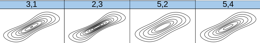
Separately, I am also using advanced statistical software to make use of a set of statistical functions called vine copulas. This part is quite geeky, and I will elaborate in a future post, but using these tools allows me to simulate environments where asset correlations change depending on the overall market environment. For example, assets can exhibit low correlation in normal times and very good times, but highly positive correlation in market crashes. Here’s an example of a set of pair copulas using five assets that have correlations that vary from good economies (top right of each graph) to bad economies (bottom right of each graph).
This advanced framework allows me to have fine-grained control over my predictive portfolio return model. Vine copula correlation models also make it much easier for Luther Wealth financial models to accommodate non-normal asset return distributions.
The LWM optimizer allows advisers (me!) to set absolute allocation limits on individual funds and securities
Often, advisers want to set floors and ceilings on individual asset allocations. The LWM optimizer has this capability. Because our proprietary optimizer is fully simulating each joint return scenario, we can set constraints on the asset weights easily. For example, I can tell the algorithm I want to maximize returns for several levels of risk, but only under the constraint that each of 10 asset classes has a minimum 5 percent allocation and a maximum 30 percent allocation.
Bottom line
Technology has improved and I want to make sure that means that YOU can benefit by having well diversified portfolios that are well suited to your personal risk tolerance.
Don’t miss out on new posts!
Don’t miss any new posts! Sign up below to subscribe. I generally post once per month and I alternate between longer-form articles and short digests of interesting financial content from other sites I’ve found. Thanks for reading!